How Private Are Private Algorithms?

The post is a $\sim$ 10 min read and only assumes knowledge about the definition of differential privacy.

We study the question in the title in the context of differential privacy, the most successful quantitative measure of privacy to date. But there are still many versions: $(\varepsilon,\delta)$, Renyi, concentrated and truncated concentrated… Which one should we use? Maybe it’s time to take a step back and see what is shared by these notions.

A good approach to providing rigorous security/privacy guarantee is by reasoning about the potential adversary:

1. What is his goal?
2. How would he achieve it?
3. How can we design algorithms so that he can’t do that?

Differential privacy (DP) can be thought of in these terms, with the following attack in mind: the adversary is given the (randomized) algorithm $M$ and its output $y$, and attempts to infer whether the input database is $D$ or $D’$. This is often called “differential attack” because his goal is to differentiate two cases.

Next question: how would he achieve differential attack? A valuable feature of DP is that it provides worst case guarantees. So we would like to think about the most powerful adversary. It turns out the most powerful algorithm to identify the input is based on a popular notion in the DP community: privacy loss.

Algorithm 1: Most Powerful Differential Attack

1. Observe outcome $y$
2. Compute privacy loss \(L=\log \frac{P[M(D')=y]}{P[M(D)=y]}\)
3. If $L>h$ then decide it’s $D’$. Otherwise decide it’s $D$.

If you can convince yourself that this is the best thing for the adversary to do, congratulations! You have rediscovered the Neyman–Pearson lemma.

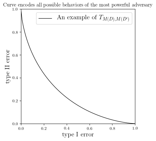
So the second question was answered 87 years ago by the founding fathers of statistics, but what we really care about is limiting the “differential power” of the adversary. In other words, we want him to make errors. The two types of errors (mistaking $D$ as $D’$, and $D’$ as $D$) are often called type I and type II errors respectively. It’s often safe to ignore which is which in DP since $D$ and $D’$ are considered symmetric. When the threshold $h$ in the above algorithm moves from $-\infty$ to $+\infty$, type I error decreases from 1 to 0 and type II error increases from 0 to 1. This yields a curve (see Figure 1) that encodes all possible behaviors of the most powerful adversary. “Differential power” would simply mean how close this curve is to the axes. Alternatively, if we consider it as a function that maps from $[0,1]$ to $[0,1]$, differential power refers to how small this function is. Because of its central importance, we will give it a name $T_{M(D),M(D’)}$ as it is determined by the distributions of the possible outcomes $M(D)$ and $M(D’)$.

A bound on differential power means guaranteed error for the adversary. To provide worst case guarantees for all possible inputs, we should consider the strongest differential power against all neighboring databases, i.e. the pointwise infimum of $T_{M(D),M(D’)}$.

Definition Differential power against a private algorithm $M$ is defined to be

At this point you may say:

Wait… I don’t recognize this sh*t… Aren’t you going too far away from differential privacy?

No, not at all.

Theorem [Wasserman-Zhou ‘10, Kairouz et al ‘15] A randomized algorithm $M$ is $(\varepsilon,\delta)$-DP if and only if the following holds pointwise in $[0,1]$

where $f_{\varepsilon,\delta}$ is defined as in the figure.

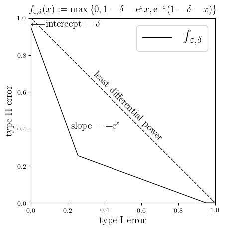
It is helpful to consider the most private mechanism $M_0$ that ignores the input and always outputs a certain distribution. Among all mechanisms, the adversary has the least differential power working against this one — he can do no better than random guessing, which corresponds to the line type I error $+$ type II error $=1$. In other words, $\Diff_{M_{0}}(x) = 1-x$. Of course, the graph (dashed line) is above that of $f_{\ep,\delta}$.

One lesson that I learned from mathematicians is, when someone tells you an inequality (for example $\Diff_M \geqslant f_{\ep,\delta}$) and you want to act like you care, ask the following

When does equality hold?

It happens to be the question in the title! That’s because, to see if equality holds, we need to know $\Diff_M$ exactly, which is a precise description of how private the algorithm $M$ is.

With the above thinking, we can start to answer the question in the title, for some “building block” private algorithms in particular. For each of them, is the true differential power $\Diff_M$ equal to the design goal $f_{\varepsilon,\delta}$? If not, how different are they?

Randomized Response: Equality Holds Exactly

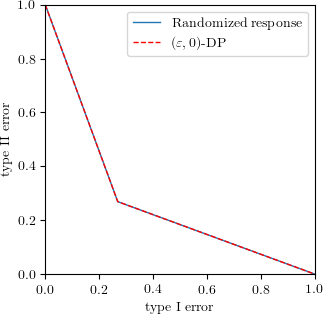
In randomized response, each individual holds one bit of sensitive information $b\in\{0,1\}$ and reports the true value $b$ with probability $p$ and its negation $\neg b$ with probability $1-p$. The randomization procedure $M:\{0,1\}\to\{0,1\}$ has the property that $M(1)\sim\mathrm{Bern}(p), M(0)\sim\mathrm{Bern}(1-p)$. When $p$ is close to 1, $M(b)=b$ with high probability. When $p=1/2$, $M(0)$ and $M(1)$ have exactly the same distribution. The easiest case for the adversary is when two bits are different, i.e.

It is well-known that $M$ is $(\varepsilon,0)$-DP if $p=\frac{\mathrm{e}^\varepsilon}{1+\mathrm{e}^\varepsilon}$. When we run Algorithm 1 (aka the likelihood ratio test) for the adversary, we can plot the differential power $\Diff_M = T_{\mathrm{Bern}(p), \mathrm{Bern}(1-p)}$ as the blue line. We see $\Diff_M = f_{\varepsilon,0}$, i.e. equality holds exactly.

Laplace Mechanism: Equality Almost Holds

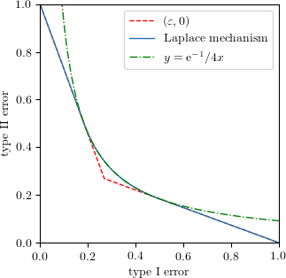
Let $q$ be a function that maps a database to a real number. Laplace mechanism $M$ adds Laplace noise $\mathrm{Lap}(0,b)$ to $q(D)$. Assuming $q$ has sensitivity 1, it is well-known that Laplace mechanism satisfies $(\varepsilon,0)$-DP if $b=\frac{1}{\varepsilon}$.

From the adversary’s perspective, he has to differentiate two shifted Laplace distributions. The easiest case occurs when $q(D)$ and $q(D’)$ differ by 1. That is, the differential power against the Laplace mechanism is

The likelihood ratio test for two shifted Laplace distributions is also easy. It turns out that in this case $\Diff_M$ mostly agrees with $f_{\varepsilon,0}$ except in the interval $[\frac{1}{2}\mathrm{e}^{-\varepsilon},\frac{1}{2}]$. In that interval it is a reciprocal function $y=\mathrm{e}^{-1}/4x$. In summary, equality almost holds.

Gaussian Mechanism: Not Even Close!

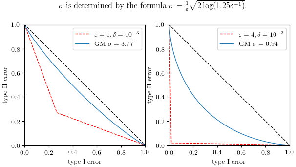
For a numerical query $q$, the Gaussian mechanism returns $N\big(q(D), \sigma^2\big)$. It was known that if $\sigma=\frac{1}{\varepsilon}\sqrt{2\log(1.25\delta^{-1})}$ then the Gaussian mechanism is $(\varepsilon,\delta)$-DP. Better formulas exist but the improvement is hardly noticeable in our context.

Similar to the Laplace mechanism, we have \(\Diff_M = T_{N(0,\sigma^2), N(1,\sigma^2)}.\) For two pairs of $(\varepsilon,\delta)$, namely $(1,10^{-3})$ and $(4,10^{-3})$, we use the formula above to determine the corresponding $\sigma$ and plot both the $(\varepsilon,\delta)$ design goal (dashed red) and the true differential power (blue). The dashed black line corresponds to perfect privacy. We see the red and blue curves are far from equal in both cases.

We proceed to examine

Composition of Building Block Algorithms

General principles of composition in DP include:

1. Composition models iterative private algorithms;
2. In terms of differential power, compostion corresponds to product distributions.

We will illustrate the two principles using randomized response as an example.

Composition of Randomized Response

Suppose each individual holds $n>1$ sensitive bits, say $b_1b_2\cdots b_n$. Each can be randomized independently. The mechanism output $M(b_1b_2\cdots b_n)$ is a product distribution. For example, assuming each bit is randomized with the same probability, then $M(101) = \mathrm{Bern}(p)\times \mathrm{Bern}(1-p)\times \mathrm{Bern}(p)$. Obviously, the adversary has the most differential power when two individuals have exactly opposite bit vectors. With a bit more argument one can show that the pair $(00\cdots0, 11\cdots1)$ is as hard as other opposite bit vectors. That is, when $M$ is a composition of randomized response, the differential power satisfies

Likelihood ratio test for Bernoulli products is also not hard. The resulting $\Diff_M$ is a piecewise linear function as the left panel shows. On the right panel we compare two mechanisms: the blue solid line corresponds to the 25-fold composition of randomized response, each being $(\varepsilon,0)$-DP with $\varepsilon=0.2$, and the red dashed line corresponds to the Gaussian mechanism with $\sigma=1$ for a query with sensitivity 1.

Clearly, something is going on here, but how general is it?

Composition of Laplace Mechanisms

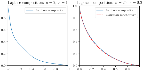
Applying the two principles, when $M$ is a composition of Laplace mechanisms, we have

This time likelihood ratio test is a bit tricky to do, but with some numerical techniques we can still do it. In the following figure, the left panel shows $\Diff_M$ for $n=2,\varepsilon=1$, while the right panel shows $n=25,\varepsilon=0.2$ and compares it again with the Gaussian mechanism with $\sigma=1$ for a query with sensitivity 1.

Composition of Gaussian Mechanisms

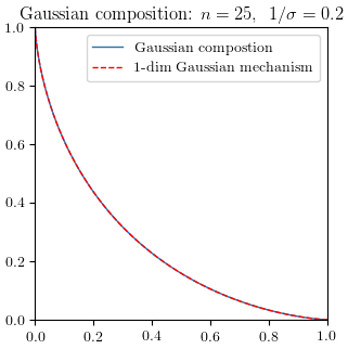
Similar to Laplace case above, we have \(\Diff_M = T_{N(0,\sigma^2)^{\otimes n}, N(1,\sigma^2)^{\otimes n}} = T_{N(0,\sigma^2 I_n), N(\mathbf{1},\sigma^2 I_n)}.\) In other words, composition of Gaussian mechanisms is reduced to testing two shifted spherical Gaussians. It is equivalent to testing shifted one-dimensional Gaussians, because a rotation can align the shifted direction to the $x_1$-axis, and the remaining components are not informative. So

Showing two identical curves is boring, but we still include the figure for completeness.

Observing these figures, we should be fairly confident that

1. There must exist a general central limit theorem, and
2. As the limit of the CLT, the differential power of 1-dim Gaussian mechanisms is something universal.

This is the origin of our paper Gaussian Differential Privacy and the deep learning follow-up. The universal object here is a single parameter family of functions

The definition of Gaussian differential privacy (GDP) parallels that of $(\varepsilon,\delta)$-DP, replacing $f_{\varepsilon,\delta}$ with the universal object $G_\mu$:

Definition A randomized algorithm $M$ is said to be $\mu$-GDP if the following holds pointwise in $[0,1]$:

GDP algorithms have a nice interpretation: Determining whether an individual’s data was used in a computation is harder than telling apart two shifted Gaussians. In addition to that, we have developed a complete toolkit for it, including theorems for group privacy, privacy amplification by subsampling and composition. More importantly, we also show the general CLT, which explains why all of the above compositions look like one-dimensional Gaussian mechanisms.

In addition to that, because 1. composition models iterative algorithms, and 2. SGD is iterative, we can apply our CLT to the most important algorithm in modern machine learning — its private version also looks like a Gaussian mechanism!

Take-away

You probably already have your own ideas, but in case that I failed to keep your attention (after all, this is my very first blog post), here is a list for your convenience:

1. Hypothesis testing is not statisticians’ perspective of DP. IT IS DP;
2. Iterative private algorithms look like 1-dim Gaussian mechanisms;
3. $(\varepsilon,\delta)$-DP does not tightly describe Gaussian mechanisms, nor any iterative algorithm.

This post is based on a talk I gave at the PriML workshop at NeurIPS 2019. Video recording can be found here, starting at 55:00. A more technical talk can be found here at Simons Institute.

15 Jan 2020